Freeze Cells in Excel allows you to lock specific rows or columns in place, making your spreadsheets easier to read and navigate. Imagine working with a large dataset, scrolling through pages of information. Freezing key rows, like headers, lets you see them clearly while you explore the rest of the data. This tutorial delves into various techniques, from basic freezing to advanced methods, dynamic freezing, and even troubleshooting.

Whether you’re analyzing financial data, managing projects, or just need to keep important headers visible while scrolling through extensive spreadsheets, mastering freezing cells in Excel is an essential skill. This comprehensive guide breaks down the process into easy-to-understand steps, from basic procedures to advanced techniques for dynamic and customized freezing. Learn how to tailor your spreadsheet layout for optimal viewing, and even how to troubleshoot any issues you might encounter.

Table of Contents

Introduction to Freezing Cells in Excel: Freeze Cells In Excel

Freezing panes in Excel allows you to keep specific rows and/or columns visible while scrolling through the rest of the worksheet. This is a crucial feature for maintaining context and preventing important information from disappearing as you navigate large datasets. It significantly improves the usability and efficiency of working with extensive spreadsheets.Freezing panes are extremely helpful for maintaining a clear overview of the data.

They enable you to constantly reference key information, like column headers or row labels, while exploring the details of the worksheet.

Freezing Panes: A Concise Definition

Freezing panes in Microsoft Excel is a function that fixes specific rows and/or columns in place while scrolling. This allows users to retain the header row and column labels, making it easier to interpret and understand data across large datasets.

Purpose and Benefits of Freezing Cells

Freezing cells enhances user experience by preventing important data from being obscured during scrolling. This maintains a clear reference point, enabling users to readily identify and analyze data across the worksheet. This significantly improves the workflow and reduces the likelihood of errors when dealing with large datasets.

Scenarios Where Freezing Cells is Useful

Freezing panes are invaluable in a variety of scenarios, enhancing productivity and minimizing errors. Consider using it when analyzing data across multiple columns and rows, for instance, when reviewing sales data across various regions and time periods, or when monitoring project progress with detailed schedules and task assignments.

Example Spreadsheet Demonstrating the Need for Freezing

Imagine a spreadsheet tracking sales figures across different regions for the last quarter. Without freezing panes, scrolling through the data to compare regional performance might be difficult and confusing. Headers like “Region,” “Product,” “Sales,” and “Date” would disappear as you scroll, making it hard to maintain context. Freezing the header row, for instance, would solve this problem, allowing you to continuously see the labels.

Table Illustrating Common Use Cases

Use Case	Frozen Rows	Frozen Columns	Benefit
Analyzing sales data by region and product	1 (header row)	1 (region column)	Allows comparison of sales across regions and products while retaining labels
Tracking project progress	1 (header row)	1-2 (task and status columns)	Maintains project overview while scrolling through tasks
Financial reporting	1 (header row)	1-3 (account, description, and value columns)	Allows quick access to financial details while viewing a large report
Data analysis across multiple categories	1 (header row)	Multiple (category columns)	Provides a reference framework for analyzing data across categories

Freezing rows and columns is a powerful tool that helps maintain data context and facilitates efficient data analysis in Excel. By freezing specific rows or columns, users can continuously view crucial information while navigating large datasets, which improves productivity and minimizes the risk of errors.

Freezing Rows and Columns

Freezing rows and columns in Excel is a powerful technique to maintain a consistent view of specific parts of a spreadsheet, especially when working with large datasets. This allows users to keep important headers or labels visible while scrolling through the data, enhancing usability and clarity. By freezing specific rows or columns, you effectively create a static reference point for your data, regardless of how far down or across you scroll.

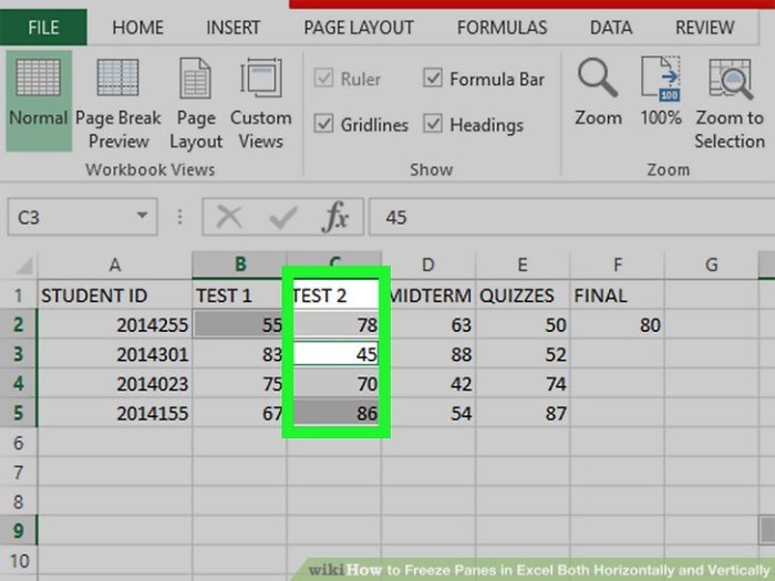
Freezing Specific Rows

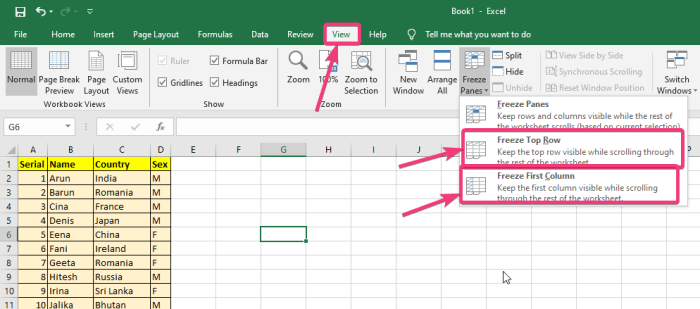
Freezing specific rows, like the header row containing column labels, ensures that those rows remain visible as you scroll down the sheet. This prevents users from losing track of the context of the data they are viewing.Freezing a single row is straightforward. Select the row immediatelybelow* the row you want to freeze. Click the “View” tab on the Excel ribbon and locate the “Freeze Panes” group.

Choose “Freeze Panes” from the dropdown menu. This action will lock the selected row (and any rows above it) in place.

Freezing Multiple Rows

Freezing multiple rows is performed similarly to freezing a single row, but instead of selecting the row

immediately* below, you select the row
immediately* below the
last* row you want to freeze. This is critical because Excel will freeze all rows above the selected row.

For instance, to freeze the first three rows, select the row directly below the third row. This ensures all rows above that selected row will be frozen, effectively keeping the top three rows static.

Freezing Columns

Freezing columns, like the first column containing identifiers or names, operates on the same principle. Freezing a column locks that column (and any columns to the left of it) in place. This is useful when working with large datasets where columns may contain important contextual information.Select the column immediately to theright* of the column you want to freeze.

Go to the “View” tab, locate the “Freeze Panes” group, and click “Freeze Panes.” This will lock the selected column (and any columns to its left) in place.

Comparing Freezing Rows and Columns

Freezing rows and columns differ primarily in their horizontal versus vertical anchoring. Freezing rows creates a static top section of the spreadsheet, while freezing columns establishes a static leftmost section. Both techniques enhance readability and maintainability when working with extensive data sets.

Freezing Top Row vs. Leftmost Column

Freezing the top row keeps header information readily available while scrolling down. The leftmost column similarly maintains crucial identifiers while scrolling across. The choice depends on the layout of your spreadsheet and the specific information you want to maintain in view.For example, a spreadsheet with product data might freeze the top row to display product names, categories, and other header details while freezing the leftmost column to display product IDs or unique identifiers.

Examples of Freezing Rows

Freezing rows is highly useful when presenting large datasets. Imagine a table with product sales figures across different regions. Freezing the top row containing region names will allow users to quickly scan sales data across different regions without losing sight of which region the data corresponds to.Another example is a student’s academic records. Freezing the top row containing the student’s name, ID, and other details enables easy identification of records while scrolling through their academic performance over the years.

Freezing Options Table

Freezing Option	Description	Impact
Freeze Top Row	Locks the top row in place.	Maintains header information visible while scrolling down.
Freeze Leftmost Column	Locks the leftmost column in place.	Maintains identifier information visible while scrolling across.
Freeze Multiple Rows	Locks multiple rows at the top.	Preserves multiple header rows or labels.
Freeze Multiple Columns	Locks multiple columns on the left.	Preserves multiple identifier columns or labels.

Advanced Freezing Techniques

Freezing panes in Excel goes beyond just the basics. Mastering advanced techniques unlocks greater flexibility and control over your spreadsheet’s layout, especially for large datasets. These methods ensure important data remains visible while scrolling through extensive rows and columns.Beyond the initial freeze, advanced techniques offer sophisticated ways to dynamically adjust the frozen area based on user interaction or automated processes.

Understanding these methods empowers you to tailor the spreadsheet to specific user needs, preventing crucial information from disappearing during navigation.

Freezing Multiple Rows or Columns

Freezing multiple rows or columns simultaneously enhances the readability and usability of spreadsheets containing large amounts of data. Instead of freezing one row or column at a time, you can freeze multiple rows or columns in a single step. This approach keeps critical headers and labels visible as you navigate through the spreadsheet. To freeze multiple rows or columns, select the cells below and to the right of the area you want to freeze.

Then, use the “View” tab, and click on “Freeze Panes”. The selected cells will remain visible as you scroll through the rest of the spreadsheet.

Dynamic Freezing Based on User Interaction

Dynamic freezing allows the frozen area to adjust automatically in response to user actions, such as scrolling or filtering. This adaptability enhances the user experience, ensuring critical information remains visible without the need for manual adjustments. Implementing this feature involves using VBA macros or formulas to monitor changes in the spreadsheet and update the frozen area accordingly. This approach is particularly useful for interactive dashboards or reports where data filters and selections frequently change.

Using VBA Macros for Automation

VBA macros provide a powerful mechanism to automate the freezing process. Instead of manually adjusting frozen panes, macros can be programmed to execute the freezing operation based on specific events, like the opening of a workbook or a change in a particular cell. This automation streamlines workflows and enhances efficiency, particularly for complex spreadsheets with multiple users or specific data manipulation tasks.

A well-designed macro can react to changes in data, automatically adjusting the frozen pane to maintain crucial headers or summaries in view.

Impact on Spreadsheet Layout

Freezing panes significantly impacts the overall spreadsheet layout. The frozen area creates a static header or label area, allowing for easy reference to specific rows and columns as you scroll through the rest of the spreadsheet. However, it’s crucial to consider the visual impact of the frozen area and ensure that it doesn’t obstruct essential data or make the spreadsheet feel cramped.

Careful consideration of the placement and size of the frozen pane is essential to maintain a user-friendly and organized spreadsheet.

Unfreezing Frozen Panes

Unfreezing frozen panes is straightforward. Simply select the “View” tab and click on “Unfreeze Panes”. This action restores the spreadsheet to its initial layout, removing the frozen area. This functionality is crucial for quickly adapting to different data viewing needs and ensuring that the spreadsheet remains flexible for various tasks.

Freezing cells in Excel is a lifesaver for complex spreadsheets. It’s like giving your data a solid foundation, making it easier to navigate and understand. Similarly, recognizing the strength in a woman, like in the article Compliment a Strong Woman , requires a thoughtful approach, which can also be quite rewarding. Ultimately, both actions, freezing cells and offering compliments, make your work and interactions more impactful and effective.

Comparison of Static and Dynamic Freezing Techniques

Feature	Static Freezing	Dynamic Freezing
Method	Manual setting of the frozen area	Automated adjustment of the frozen area based on user interaction or formulas
Flexibility	Limited; fixed frozen area	High; adjusts automatically to changes
Complexity	Simple; requires basic understanding of Excel	Moderate; involves VBA or advanced formulas
Use Cases	Basic data analysis, fixed headers	Interactive dashboards, dynamic data summaries

Dynamic freezing offers greater flexibility for interactive spreadsheets. However, static freezing is often sufficient for simple data analysis tasks.

Freezing cells in Excel is a game-changer for complex spreadsheets, just like crafting a magnificent dinosaur tail requires careful planning. Imagine needing to reference a specific header row while working on extensive data. Learning how to freeze cells in Excel allows you to keep those headers visible as you scroll through the data. It’s like having a constant reference point, just like the detailed construction process in making a dinosaur tail from Make a Dinosaur Tail.

Mastering this Excel trick saves time and frustration, making any spreadsheet project more manageable.

Freezing Cells with Data Validation

Freezing cells containing data validation rules ensures that the validation settings remain consistent and visible to the user. This is particularly important in interactive spreadsheets where users need to make choices based on predefined options, preventing accidental modification of critical validation settings. This method enhances the predictability and consistency of user input.Freezing validation cells, like other frozen cells, keeps them static while the rest of the sheet scrolls.

This makes the validation rules readily accessible and avoids the user having to constantly reposition their view. This approach is crucial when working with complex spreadsheets containing numerous validation rules.

Freezing Cells with Drop-Down Lists

Freezing cells containing drop-down lists within a data validation rule is a standard practice for maintaining the integrity of user input. This ensures that the available options remain visible, even as other parts of the spreadsheet are scrolled. Users can always see the predefined options and select the appropriate one without having to repeatedly reposition the view.

Freezing Cells with Input Fields

Freezing cells with input fields, such as text boxes or number fields, is crucial for ensuring that data entry adheres to predefined formats and constraints. This prevents users from accidentally changing the input rules. Freezing these cells ensures the user sees the validation rules and the correct format or range of values for the input field.

Examples of Critical Applications

Freezing cells with validation rules is essential in various scenarios. A crucial example is in a sales order form. Freezing cells with product categories, quantities, or unit prices, each with predefined validation rules, ensures that users select valid options. This prevents the entry of incorrect data, improving data accuracy. Another example is in a survey or questionnaire, where freezing cells containing answer choices ensures that users select only the pre-defined options.

Effects on User Input

Freezing validation cells significantly impacts user input by improving data accuracy and predictability. Users can quickly identify the validation rules and constraints associated with each cell. This clarity and ease of access reduces errors and ensures data integrity.

Creating an Interactive Table with Frozen Validation Cells

A well-designed table with frozen validation cells can create a highly interactive spreadsheet. The table should be structured logically, with validation cells frozen for easy user access. For example, a table for tracking expenses might have columns for expense type, amount, and description. The expense type column could use a drop-down list validated against a predefined list of expense categories.

Freezing this column ensures users can always see the options available. The amount column might have a validation rule limiting the input to numeric values within a certain range. Freezing this cell ensures that the user understands the rules.Consider using conditional formatting to highlight cells that violate the validation rules. This visual cue further enhances the interactive experience and aids in data entry accuracy.

Troubleshooting Freezing Issues

Freezing panes in Excel can sometimes present unexpected challenges. Understanding common errors and their solutions can save you significant time and frustration. This section dives into troubleshooting techniques for various freezing scenarios, ensuring your spreadsheets remain functional and well-organized.Excel’s freezing feature, while straightforward, can encounter problems if not used correctly or if other factors interfere. Identifying the root cause is crucial for effective troubleshooting.

Freezing cells in Excel is a super handy feature for maintaining a clear view of your data, especially when dealing with large spreadsheets. It’s like having a constant reference point while you scroll through rows and columns. Speaking of important recognitions, I was really impressed to hear that Mavis Staples, The Eagles, and James Taylor are all going to receive the Kennedy Center Honors! This incredible news reminds me that sometimes a little recognition is all you need to keep your spreadsheets organized, much like how freezing cells keeps important data visible while you’re analyzing the rest.

Freezing cells is just one of those simple, yet powerful, Excel tricks that can transform your workflow.

Common problems include incorrect cell selection, conflicting settings, or even unexpected Excel crashes during the freezing process.

Common Freezing Errors and Solutions

Incorrect cell selection is a frequent cause of freezing pane issues. If the selection doesn’t precisely encompass the desired rows and columns, the freezing will not function as intended. Carefully reviewing the selected range before activating the freeze pane is vital.

Incorrect Selection: Ensure the selected range accurately reflects the rows and columns you want to freeze. Select the cells above and to the left of the area you want to lock. If only a single cell is selected, the entire row and column will freeze. Using the mouse to drag and select the area is often the easiest method.
Conflicting Settings: Other Excel features or add-ins might interfere with the freezing process. Ensure no other processes are active or that other extensions aren’t overriding the freezing settings. Temporary disabling of potentially conflicting add-ins can often resolve the issue.
Unexpected Excel Crashes: Sometimes, Excel unexpectedly crashes while freezing panes, leading to data loss or incomplete freezes. This can stem from issues with the spreadsheet’s formatting, or the system’s resources. Saving the file frequently and ensuring sufficient system resources are available (memory and processing power) can help mitigate this risk.

Troubleshooting Techniques for Different Scenarios

Different scenarios require tailored troubleshooting approaches. A systematic process can effectively pinpoint the cause of the problem.

Repeated Attempts: Try freezing the panes multiple times if the initial attempt fails. A second or third try might fix temporary glitches. If the problem persists, the issue might lie elsewhere.
Restart Excel: A simple restart of Excel can often resolve minor glitches. This can clear temporary files or settings that might be causing conflicts.
Reviewing Formulas: Complex formulas in the sheet can sometimes interfere with freezing panes. Examine any formulas in the cells adjacent to or within the area being frozen, looking for possible errors or inconsistencies.

Table of Common Problems and Solutions

The following table provides a quick reference for common freezing issues and their resolutions.

Problem	Solution
Freezing panes not working correctly	Verify the selected range and ensure no conflicting add-ins or processes are running.
Excel freezing unexpectedly during the process	Save the file frequently, ensure sufficient system resources, and review formulas in the affected cells.
Incorrect area frozen	Correctly select the cells above and to the left of the area you want to freeze.

Freezing Cells in Different Excel Versions

Freezing cells in Excel is a powerful feature that allows users to keep certain rows and columns visible while scrolling through the rest of the worksheet. This is crucial for maintaining context when dealing with large datasets. Understanding how this feature operates across different Excel versions is important for seamless workflow and data analysis.Excel’s freezing capabilities have evolved over time, introducing subtle changes and enhancements in different versions.

While the core functionality remains consistent, variations in the user interface and specific options can influence how you achieve the desired freezing effect.

Excel 2010 Freezing Method

The freezing method in Excel 2010 primarily involved using the “Freeze Panes” feature within the “View” tab. Users could choose to freeze rows or columns from the top or left edge of the worksheet. This method is straightforward but lacked some of the flexibility available in newer versions. The process was primarily manual and required direct interaction with the Excel interface.

Excel 2016 Freezing Method

Excel 2016 retained the fundamental “Freeze Panes” feature. However, the user interface offered slightly improved options and control over the freezing process. Users could freeze rows and columns, as well as specify which panes should remain fixed. The options for freezing were more intuitive than in 2010, making it simpler to accomplish specific freezing layouts.

Excel 365 Freezing Method

Excel 365 built upon the previous versions’ features, providing a more comprehensive and customizable approach to freezing cells. Users gain the ability to freeze panes with a more interactive and precise method, directly influencing the display and scrolling behavior of the worksheet. Advanced options allow for more complex freezing arrangements.

Compatibility Issues and Changes

While the core concept of freezing cells remains consistent across versions, some minor compatibility issues might arise when working with files created in older versions within newer versions of Excel. These differences mainly concern the display and accessibility of specific freezing options, but rarely affect the functionality itself. The newer versions often provide enhanced user interface options, making the process more intuitive.

Users opening older files might need to adjust their settings to match the original layout, although it’s usually a straightforward process.

Summary Table

Excel Version	Freezing Method	Key Features	Compatibility Notes
Excel 2010	“Freeze Panes” feature, manual selection	Basic freezing of rows and columns.	Works well within 2010 but may require adjustments when opened in newer versions.
Excel 2016	“Freeze Panes” feature, improved interface	Enhanced user interface, precise control over frozen panes.	Works seamlessly with 2010 files, though UI may differ slightly.
Excel 365	“Freeze Panes” feature, advanced options	Highly customizable freezing arrangements, intuitive UI.	Full compatibility with 2010 and 2016 files, with improved user experience.

Customizing Frozen Cell Appearance

Freezing cells in Excel is a powerful feature for maintaining a consistent view of critical data. However, the default appearance might not always suit your specific needs. This section explores various methods for customizing the visual presentation of your frozen cells, making them stand out, easier to read, and better integrated with your worksheet’s overall design.Beyond the basic freeze panes, enhancing the appearance of frozen cells allows for improved readability and a more visually appealing spreadsheet.

This includes altering colors, fonts, and borders, and employing conditional formatting to dynamically highlight certain frozen cell values based on specific criteria.

Formatting Frozen Cells

Customizing the appearance of frozen cells is straightforward and offers significant advantages for data presentation and analysis. Applying different formatting options can greatly enhance the visual appeal and usability of your spreadsheet. This section covers the fundamental formatting options that can be applied to frozen cells.

Font Formatting: Change the font style, size, color, and effects (bold, italic, underline) of the frozen cells to improve readability. For instance, you might choose a bold, larger font size for crucial metrics in the frozen row header, or a distinct color to highlight specific data points. The selection of the appropriate font attributes depends on the context of the data and the overall design aesthetic of the spreadsheet.
Cell Fill Color: Apply a fill color to frozen cells to make them visually distinct from the surrounding cells. A subtle color gradient or a solid color can be used to differentiate the frozen cells, providing visual cues and making them easily recognizable. For example, a light blue fill color can be used to highlight the frozen row containing column headers, making them stand out and easily identifiable.
Border Formatting: Adding borders to frozen cells helps to define their boundaries and enhance their visual clarity. This could include varying line styles, colors, and thicknesses. For example, a thicker, darker border can be used for the frozen column headers to clearly separate them from other cells in the same column.

Conditional Formatting of Frozen Cells

Applying conditional formatting to frozen cells allows for dynamic highlighting based on the values within those cells. This feature is highly useful for quickly identifying trends or anomalies.

Highlighting specific values: Use conditional formatting to highlight frozen cells that meet certain criteria, such as cells containing specific values, exceeding or falling below a certain threshold, or showing a particular trend. For example, you might highlight frozen cells containing sales figures that exceed the monthly target. This instantly draws attention to important data points.
Color scales: Employ color scales to highlight data ranges in frozen cells. This allows for a quick visual representation of the data distribution. For instance, a color scale can be used to show the performance of different products, with different colors corresponding to different sales ranges. This provides a concise visual summary of the data.
Data bars: Use data bars to represent the magnitude of values in frozen cells. This visual representation is helpful for quickly comparing the relative sizes of different values. For instance, data bars in frozen cells can highlight the sales performance of different regions, with bars of different lengths representing the different sales figures.

Formatting Options Table

Formatting Option	Description	Example
Font Style	Bold, italic, or other font variations	Bolding column headers in the frozen row
Font Color	Change the color of the font	Highlighting critical data points with a specific color
Cell Fill Color	Apply a background color to the cell	Using a light gray fill for the frozen row headers
Border Style	Adjusting border thickness and color	Adding thicker borders to the frozen columns
Conditional Formatting	Highlighting cells based on rules	Highlighting cells containing values exceeding a target

Freezing Cells in Specific Situations

Freezing cells in Excel isn’t just a cosmetic touch; it’s a powerful tool for enhancing spreadsheet readability and usability, especially in complex analyses. By strategically freezing specific rows and columns, you can maintain a consistent header view while exploring data across numerous rows and columns. This approach is particularly valuable in financial modeling, project management, and data analysis where navigating extensive spreadsheets is common.Freezing cells isn’t a one-size-fits-all solution.

The optimal approach depends heavily on the specific data structure and the analysis being conducted. Understanding these nuances will help you leverage freezing effectively, improving your workflow and enabling better insight into your data.

Financial Analysis Examples

Freezing cells is invaluable in financial modeling. Imagine a spreadsheet detailing monthly revenue and expenses for a company. Freezing the header row allows you to track the month-to-month variance while easily comparing different categories. Freezing the first column, containing product names or project IDs, lets you maintain a clear view of the item while analyzing the details in other columns.

Project Management Applications

In project management, freezing cells can be just as helpful. A project timeline, for example, might have tasks listed across columns and durations in rows. Freezing the top row (containing the task names) and the first column (for the date ranges) provides a consistent reference point as you scroll through the project schedule.

Optimal Freezing Methods for Different Data Structures

Choosing the right freezing method hinges on the spreadsheet’s structure. For tabular data, freezing rows and columns based on header information is often the most practical approach. For complex, interconnected datasets, a combination of row and column freezing might be required to keep critical elements visible while exploring other details.

Organizing Spreadsheets for Enhanced Visualization

To maximize the benefit of freezing cells, organizing the spreadsheet with clarity is paramount. Clearly defined headers, appropriate formatting, and a logical arrangement of data will make the frozen cells more effective in guiding the user.

Specific Situations and Optimal Freezing Techniques, Freeze Cells in Excel

Situation	Optimal Freezing Technique	Description
Financial Statements (Monthly Revenue/Expense)	Freeze header row and first column	Maintains header visibility while analyzing data for each month and category.
Project Timeline (Tasks vs. Dates)	Freeze header row and first column	Provides a consistent view of tasks and dates while scrolling through the project schedule.
Sales Data Analysis (Products vs. Regions)	Freeze header row and first column	Enables comparison of sales figures for different products in various regions.
Inventory Management (Products vs. Locations)	Freeze header row and first column	Allows for efficient tracking of inventory levels across different product categories and locations.

Ending Remarks

Freezing cells in Excel elevates your spreadsheet experience, allowing you to work more efficiently with large datasets. This guide has provided a clear roadmap for understanding and applying various freezing techniques. From basic freezing to advanced dynamic methods and even considerations for different Excel versions, this comprehensive guide equips you with the knowledge to optimize your spreadsheet layouts for any situation.

Now you’re ready to master your Excel spreadsheets, one frozen cell at a time!